| THE INTEGRITY PAPERS | Genre Group | ceptualinstitute.com/genre.htm |
BIOS: Creative Organization Beyond Chaos
Louis H. Kauffman and
Hector Sabelli
There are several special aspects about BIOS dynamics that you will be reading here.
|
Louis H. Kauffman and
Hector Sabelli
University of Illinois at Chicago
851 South Morgan St., Chicago, Illinois 60607-7045
e-mail: <kauffman@uic.edu>
a n d
Chicago Center for Creative Development
2400 Lakeview, Chicago, Illinois 60614
e-mail: <hsabelli@rpslmc.edu>
Paper prepared 1997/8. Int'l Soc for Systems Sciences presentation, 1998.
Summary:
Bios is a new type of organization characterized by the continual generation of novel patterns. Bios thus provides a new concept regarding physiological regulation and creative evolution. Different types of biotic patterns have been found in physiological and economic time series, and can be generated by the process equation A(t+1) = A(t)+ g t sin(A(t)) that models the diversity of positive and negative interactions to be expected from the environment. In investigating fundamental process we are looking for elemental pairs of opposites living in creative dialogue. The process equation exemplifies this approach and it provides a compass for the investigation.Key words:
bios, process, recursion, pattern, creation, novelty.1. Introduction
In this paper we report on a mathematical pattern that we call bios, a variant of chaos identified in heartbeat intervals and also by an equation that we dub the process equation [Kauffman and Sabelli (1998)], [Sabelli and Kauffman (1999)].
The process equation generates convergence to
p , a cascade of bifurcations, chaos, bios and infinitation, according to the value of the feedback gain g. When g is a linear or sinusoidal function of time, the bifurcation diagram generates "lifeforms" that evolve from one fixed point ( the "egg" in this organic metaphor) through a cascade of partitions into bios, and end in infinitation. In the complex plane, numerical series generated by orthogonal (sine and cosine are orthogonal) process equations display fractal organic patterns .This paper is organized as follows: Section 2 discusses the process equation and its relation to chaos and bios. Section 3 discusses mathematical properties of the process recursion. Section 4 discusses the relationship of the process equation to the circle map studied in the literature of chaos theory. Section 5 discusses variations on the process equation. Section 6 discusses complement plots of biotic series. Section 7 is a short remark on process theory. Section 8 summarizes the paper.
Acknowledgement.
It gives Kauffman great pleasure to thank the National Science foundation for support of this research under NSF Grant DMS-9802859 and the National Security Agency for support of the research under grant MDA904-97-1-0015. Sabelli thanks the Society for the Advancement of Clinical Philosophy for support during the preparation of this paper.
2. The Process Equation
The purpose of this section is to draw attention to a number of remarkable properties of the recursion
A(t+1) = A(t) + gsin(A(t))
where the A(t) are real numbers. We call this equation the
process equation. We call the value g the gain of the process equation.For small gain near zero the recursion tends to the fixed point A=p. As g is increased there is a series of bifurcations or apparent bifurcations, for as is evident in Figure 1 there are places where the process changes its character and appears to have the form of bifurcation without the substance of the appearance of a new branch. This unifurcation is one of the new phenomena to which we refer.
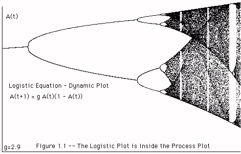
As g becomes sufficiently large there is a transition to chaos, analogous to that in the logistic equation
A(t+1) = gA(t)(1 - A(t)).
However in the process recursion we have the abrupt "walls" apparent in Figure 1. These walls are never seen in logistic chaos. The most startling phenomenon, however, occurs at about g=4.605 (near the Feigenbaum constant) where the process continues (as opposed to the logistic equation) and acquires a new character that we call "biotic". In this biotic phase (g > 4.605) the process has many similarities to biological time series, particularly to heartbeat data. Biotic series, but not chaotic series show the following features that also obtain in heartbeat series: (1) episodic patterns ("complexes") separated by relatively patternless transitions; (2) recurrence rate lower than random.
A detailed picture of the biotic pattern in given in the next sections.
3. Thinking about the Mathematics of the Process Equation
We study graphic plots related to the process equation in three ways that we call the dynamic plot, the kinetic plot and the dynamic seed plot. In the dynamic plot the gain is a step function of time, so that we can gather a list of successive values of the recursion for a fixed value of the gain. In the kinetic plot the gain increases by a small increment with each time step. In the dynamic seed plot, gain is held fixed for periods of time and the same initial value is entered for the recursion each time the gain is increased. Each of these methods reveals different (although related) information about the structure of the process recursion. The kinetic and dynamic plots give a very similar appearance when the gain increment of the kinetic plot is very small. Nevertheless subtle differences occur in the comparison of these methods.
Strictly speaking, the kinetic plot should be regarded as the plot of a different process than the dynamic plot. In the kinetic plot the equation of process is
A(t+1) = A(t) + g(t)sin(A(t))
where the gain g(t) is a function of time. We usually take
g(t) = c + t
Dwhere c is a starting value for the gain and
D is a small constant. The kinetic plot then plots the points (t, A(t)). If D is small in relation to the size of the increment of t, the kinetic plot will resemble the dynamic plot, but generates additional phenomena.We also use
cobweb plots (described below) to illustrate and investigate the process dynamics.In Figure 1 we show a dynamic plot of the process equation. The vertical axis plots A(t) for many (200) values of t and a fixed g where g is the value of the horizontal coordinate. For a given g this plot shows when A(t) is a fixed point (or steady asymmetry), periodic point, chaotic or biotic. By looking back and forth along the plot the reader can see how the process equation changes as g changes its value. This dynamic plot is made by running the process equation, plotting points for a given value of g, then increasing the value of g (by 0.01) and running again. This means that the seed value of A for a new value of g is obtained from the last value of the previous run of the recursion.
Remarkably,
we can experimentally verify that the dynamic plot of the logistic equation occurs inside the dynamic plot of the process equation. View Figure 1.1.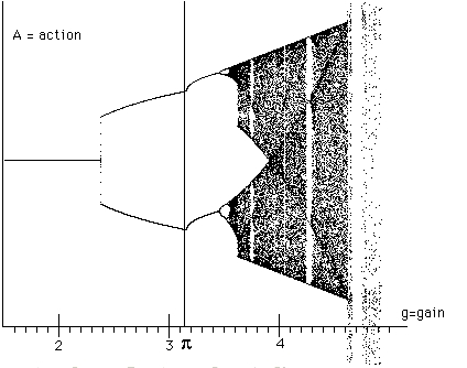
Figure 1 -- Process Equation -- Dynamic Plot
In the graph for Figure 1, we have drawn a vertical line at the value where the gain is equal to
p. Notice the unifurcation phenomenon at g=p. The period two points in the full plot suddenly move "upward" together, and it looks like there could have been a downward branching as well. It is a computational fact that this phenomenon occurs at g=p. While we have no other proof of this fact at this time, the following discussion is quite suggestive.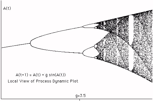
Note that phenomena viewed using large increments in the stepping of the gain g can occur at different values of the gain than the corresponding phenomena in the same series with small increments.
Can we understand the reason for the unifurcation?
Why would the process appear to bifurcate but not show a branch of the bifurcation? We see the dynamics of this by using a cobweb plot. The picture below (Figure 2) shows the structure of the cobweb plot for the process equation in the neighborhood of the unifurcation.
In the case of the unifurcation, we find that it shows up in the cobweb plot as described below. The cobweb has the advantage of showing visual dynamics of this part of the process.
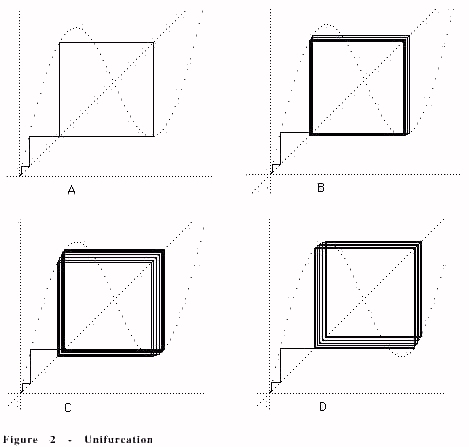
Each plot has a constant g. The plot has a dotted wavy figure that is the graph of y=f(x)= x +g sin(x) where x denotes the horizontal axis and y denotes the
vertical axis. We draw lines from(x,x) to (x,f(x)) and from (x, f(x)) to (f(x), f(x)).
The iterates of the function f(x) appear as the off-diagonal points in the cobweb.
Returning to the plots in Figure 2, we illustrate an increasing sequence of values of g in subfigures A, B, C, D. We see that at A the cobweb plot indicates a period two pattern as indeed one sees in the plot of the process equation shown in Figure 1. As g is increased to D this period two vibration shifts to a
larger value, but remains at period two. This is the first instance of unifurcation. It is clearly (from the cobweb plot) a consequence of the weaving back and forth between the maximum, minimum and "walls" of the sine wave pattern in the graph of y=x+gsin(x).Most importantly note that the basic shift is a movement where the period four pattern moves from using the right-hand lower minimum of the graph to using the left hand upper maximum of the graph. See the bottom two pictures in Figure 2.
This brings us to a further discussion of the pattern of unifurcation in the process equation plot as discussed in relation to Figure 1. It is not hard to see that this pattern has a mathematical "mate" that fits together with it to form a simulacrum of bifurcation. One way to find the mate is to use a deformed process equation as in
A(t+1) = A(t) + g sin( A(t) +
q ).If
q is chosen appropriately then we can get a situation where a slight decrement of q leaves the pattern alone but a slight increment gives the mate. This pivot point appears to be quite exact. In Figure 3 we exhibit this phenomenon with q = 2.71795 (down) and q = 2.71796 (up).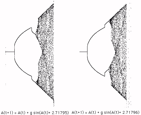
Figure 3 - The Pivot Between UpWalls and DownWalls
In the pivot example shown in Figure 3 we have a new example of sensitivity to initial conditions where we regard the value of
q as an initial condition for the recursion. (The examples start with x = p) The global configuration of the process equation plot is affected by infinitesimal changes in this initial condition.Another way to create a mate in the dynamic plot is to use a different initial condition. We used the initial condition A(0)=0.001 to produce the plot in Figure 3. If we use A(0) = -0.001 (starting from a small negative value) then the mate will appear, with the unifurcations going downward rather than upward. In the first instance the process converges to the fixed point at A =
p. In the second instance the fixed point is A = -p. As the gain is increased the fixed point becomes unstable and the branching in the dynamic plot begins. Of course it is the computational error in the computer that allows the bifurcation to begin. If the computer were mathematically perfect, then the process would remain at the fixed point!Now lets turn to the next phenomenon in the dynamic plot of the process equation. This is the actual bifurcation to period four at around g=3.5. Figure 3 shows the cobweb plot for g=3.5. We see the exact form of the period four and how it involves a "bounce" among the sides of the little reflection space made by one maximum and one minimum of the sin function distorted into y = x +gsin(x).
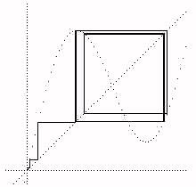
Figure 4 - Period Four at g=3.5
Continuing the tour of the full plot, we arrive at the strange "walls" at around g=3.6. Here the plot suddenly acquires a larger chaotic component. It goes from chaos to larger chaos abruptly. Now look at the cobweb plot in Figure 5.
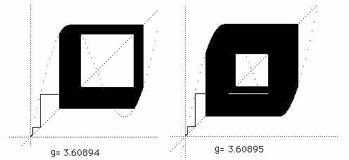
Figure 5 - The Onset of the Wall
In Figure 5 we see how chaos at g=3.60894 suddenly becomes larger chaos at g = 3.60895. Again this a property of the y=x+gsin(x) reflection space. Finally in Figures 6 ,7 and 8 we see the cobweb plots that illustrate the transition from chaos to bios. In this transition the dynamics that was restricted to a "reflection space" consist- ing of one maximum and one minimum of the graph y=x+gsin(x) suddenly "breaks out" and begins a complex motion in a larger space. We will later look at more details of this process. We call this break out phase bios.
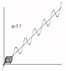
Figure 6 - Pre Biotic Phase
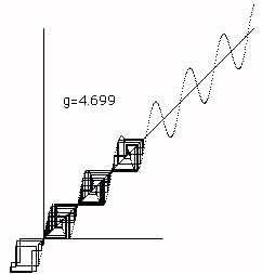
Figure 7 - Transition to Biotic Phase
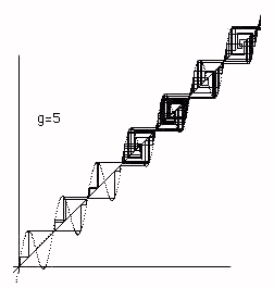
Figure 8 - Biotic Phase
The next topic we take up is the appearance of the process equation dynamic seed plot. In the plot below (Figure 9), we use a seed value of A=0.0001 and start at this value for each choice of g.
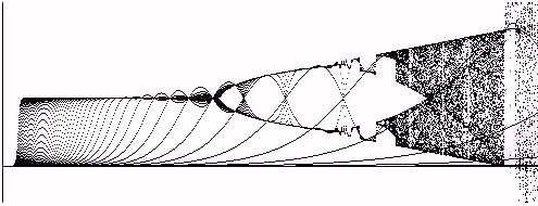
Figure 9 -- The Dynamic Seed Plot with Seed = .0001
With the seed near zero we see that zero is an unstable fixed point for the process from the very beginning. In contrast,
p is a mathematical fixed point at the beginning and we get the dynamic seed plot with transients as shown in Figure 10.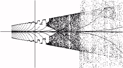
Figure 10 - Seed = p
In Figure 10 we have drawn a vertical line at g=p for comparison with Figure 1. More work is needed to understand these phenomena.
Recurrence Plots and Bios
Another feature of the biotic phase stands out in recurrence plots of the time series. A recurrence plot is obtained from a time series A(t), for the "times" t=1,2,3,...as follows: Choose a vector dimension d and associate a vector V(t) to each time t by the equation
V(t) = (A(t), A(t+1), A(t+2), A(t+3), ..., A(t+d-1)).
The norm of a vector v, denoted ||v||, is the square root of the sum of the squares of the components of v. One may compare vectors v and w by taking the norm of their difference, ||v-w||. For each pair of vectors V(t), V(t') we compute ||V(t) -V(t')||. If this norm of the difference is less then C for a chosen criterion C, plot a point at (t,t') in the Time x Time plane. The resulting recurrence plot gives a graphic picture of the self-correlation of the original time series, and it provides a fertile domain for experimenting with such patterns of self-correlation. See Figure 11 for an example of a recurrence plot for the biotic phase of the process equation. In this figure the total length of the time series is 300, the vector length is d = 10 and the criterion for plotting is C = 20.
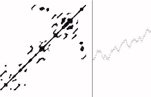
Figure 11-- Process Equation, g=4.9 Recurrence Plot
In Figure 11 we have shown the time series on the right half and the corresponding recurrence plot on the left half (separated by a vertical line). A number of results can be seen from these plots. First of all, there is a concen- tration into localized complexes as shown in Figure 11. These complexes are characteristic of bios, and can be understood in the process equation as related to the patterns of repeated visiting to regions of paired maxima and minima in the graph of y = x + g sin(x).
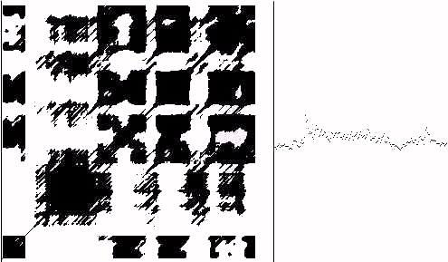
Figure 11.1 - Heart Data -- Recurrence Plot
In Figure 11.1 we show a recurrence plot of heartbeat interval data using a similar set of parameters, 300 points in the time series, vectors of dimension 10 and C = 20. It is quite interesting to compare the qualitative and quantitative features of the heartbeat data with bios. In the case of both Figures 11 and 11.1, the choice of criterion C is dependent on the range of values of the series. Different values of C can bring out different aspects of the recurrence.
If one shuffles the time series and makes the recurrence plot again, the shuffled plot will have a more uniform distribution of recurrences, without the concentration into domains that is seen in bios as in Figures 11 and 11.1.
One also sees that for process equation bios, the shuffled plot has
m o r e recurrences than the unshuffled plot.In other words
the incidence of recurrence is lower in bios than in random. We take this as an indication that the biotic pattern is exhibiting n o v e l t y . A series with low recurrence rate is regarded as having novelty while high recurrence as in periodic patterns signifies the lack of newness. This notion of novelty has two purposes. On the one hand it provides an operational definition of novelty. On the other hand it gives us a chance to raise the issue of the nature of novelty in more general contexts. That discussion will be taken up in other publications. Let us only note here that these changes with shuffling are exactly the same as those that happen with the heart.
4. The Circle Map
A mapping that is related to the process equation can be obtained by taking
A(t+1) = A(t) + g sin( A(t) ) (Mod P)
for an appropriate period P. In the literature this is called the circle map and has been much studied for P= 2p.
Remark.
The circle map most commonly studied has the formA(t+1) = A(t) + 2
pW + K sin(A(t) + d).(See [Froyland (1992)], [Glass and Mackey (1988)].) Many phenomena (such as the Arnold tongues [Froyland (1992)]) occur even with K=0. Here we relate the process equation to the circle map in the case where
W=0 . The phenomena that we have been discussing in relation to the process equation are not available or are hidden in the circle map. In particular the biotic phase is not visible in the standard circle map due to the mixing that occurs from the modulus. Some other process equation features appear transiently in the beginning of the circle map. In Figures 12 and 13 we show the beginnings of the circle map with P=3 in Figure 12 and P= 2p in Figure 13.Note the transient cascade in Figure 12 and note that we see the process equation chaos reproduced at the beginning in Figure 13. There are other chaotic bifurcation patterns in both figures that bear a resemblance to the chaos of the logistic equation, but it is clear that these are actually coming from the process equation folded into itself from its different appearances emanating from the fixed points of sin(A) at different multiples of
p. Of course these folded appearances of "fake" logistic process should be compared with the actual logistic process. This will be the subject of another paper.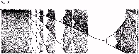
Figure 12 -- Mod 3 Cascade
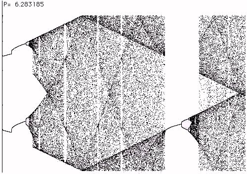
Figure 13 -- Mod 2
p - Process Equation Dynamics in the Circle Map5. Variations on the Process Equation
There are many variations that one can make on the basic process equation discussed in this paper. In this section we will mention a few of these and discuss their properties.
The Sabelli Attractor
A(t+1) = A(t) + B(t) cos(A(t))
B(t+1) = B(t) + A(t) sin(B(t))
Here are the equations of a self-contained two dimensional process consisting in two interlocked process equations where the gain of each equation is the output of the other equation. This mutuality gives rise to a very beautiful attractor as illustrated in Figure 16.
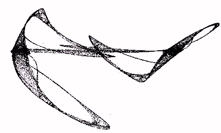
Figure 16 - The Sabelli Attractor
Note that the set of points in the Sabelli attractor is invariant under the mapping of the plane to the plane given by the equation F(A,B) = (A + B cos(A), B + A sin(B)). Note that this strange attractor is produced by the mutual control of gain in these equations.
Of course the Sabelli attractor has variations of its own, and we leave that subject to another paper.
Cocreating Equations
A(t+1) = A(t) + g B(t) Sin(B(t))
B(t+1) = B(t) + h A(t) Cos(A(t))
We call this next variation "cocreating equations". In the cocreating equations there are two linked process equations, but in each equation the gain and feedback comes from the other one. For specific values as shown below
Initial values A=6.3734761, B=.00001.
A(t+1) = A(t) + .1 B(t) Sin(B(t))
B(t+1) = B(t) + .01 A(t) Cos(A(t))
we get a most extraordinary sequence of events [Sabelli, Kauffman, Patel, Sugerman, Carlson-Sabelli, Afton, and Konecki (1997)] as shown in Figures 17, 18 and 19. In these figures we have shown the results of the organic pattern that emerges from the recursion at successive levels of magnification.
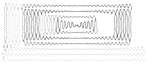

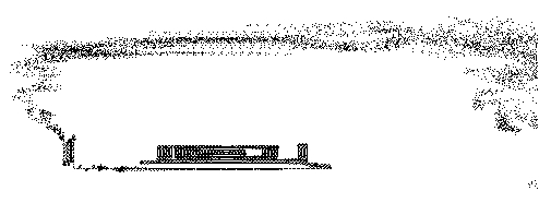
Figure 17 - First Steps ... from 'seed' to 'smoke'
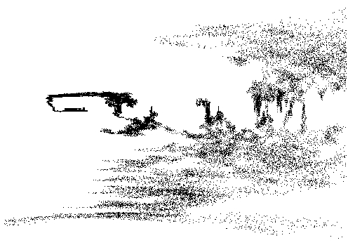
Figure 18 - Stepping back
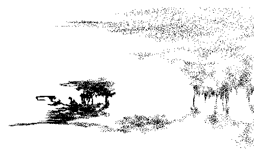
Figure 19 - Stepping Farther Back
At the very first level we see the stage of the "seed" where there is a slow transition working its way through a two dimensional oscillatory process that starts to build a two dimensional chaotic region. Eventually, the process breaks out into bios in the form of the wandering smokelike path in two dimensions that continues at many scales above the beginnings of the process. In the course of these wanderings, forms are painted and it is the production of these forms that leads us to call these linked equations the cocreators of organic forms. The forms that are seen result from the clustering behaviour of this process. This generation of forms with similarities at many levels of the recursion goes beyond bios to a new process closely allied to the organic nature of our universe.
6. Complement Plots
Let A(t) be any time series. Plot in the plane the points
( cos(A(t)) , sin(A(t)) ) .
This is the
complement plot. The complement plot was created to reveal the coexistence of opposites when only one time series was available. This is accomplished by composing the single time series with both the sine and the cosine in this manner. We obtain patterns that reveal much about many processes. Mandala - like patterns appear for the heart [Sabelli (1999)]. In Figure 20 we illustrate the complement plot for the process equation with gain g=4.0. Notice that there is a gap in the circle. This is characteristic of the complement plot of the process equation prior to the biotic phase. In Figure 21 we show the complement plot for the process equation with gain g=4.8. Now the circle has closed. This contrast between the closed and open circles can be seen correspondingly in the cobweb plots where the area between the first minimum and first maximum of the cobweb plot graph is not filled completely until the onset of bios.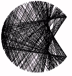
Figure 20 - Process Complement Plot -- g = 4.0
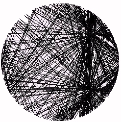
Figure 21 - Process Complement Plot -- g = 4.8
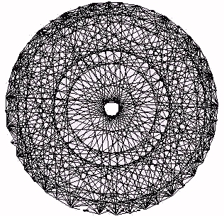
Figure 22 - Heart Data Complement Plot
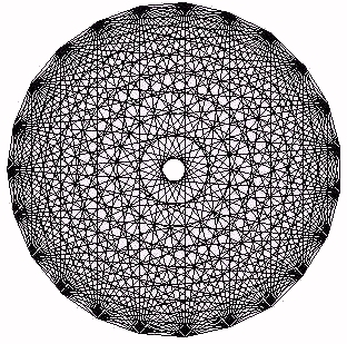
Figure 23 - The Complete Graph on 23 Vertices
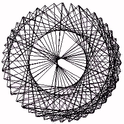
Figure 24 - Process Equation - Integer Complement Plot g=4.8
In Figure 22 we show the complement plot of heartbeat intervals (these data have integer values). Note how the plot produces a set of concentric ring patterns in a mandala - like form. This plot of heartbeat data is not at all like the Figure 21 plot of process bios. The source of this discrepancy is the fact that the bios recursion does not produce a series of integers. In Figure 24 (at a different unit scale) we show the result of making an integer complement plot
for the process recursion at g=4.8. If A(t) denotes the values of the process recursion, we have then plotted (cos(Int(A(t)), sin(Int(A(t))) for many values of t, where Int(x) denotes the greatest integer in x. This plot of process bios does have a pattern similar to the complement plot for heartbeat intervals.In Figure 23 we illustrate the complement plot obtained by connecting all possible chords between 23 equally spaced points around a circle. It is worth comparing this "ideal" circle plot with the results in the other figures. Note how the heart data selects only some of the concentric rings that appear in an ideal plot. This selectivity becomes a footprint for the process being studied.
Cardiac biotic series generate a pattern of concentric circles in complement plots [Sabelli (1999)]. Equation-generated biotic series rounded to integers generate Mandala patterns similar to those of the heart. Chaotic series (process or logistic equation) generate partial circles that reduce to simple figures when the data is rounded. The process time series turns into a biotic Mandala when the circle of opposites is closed. Even after closing the circle; there remains an asymmetry (see Figure 24). Sine and cosine are paradigmatic of complement- ary opposites. They co-create the circle, and so we come full circle to the information space in which this method is based.
7. Process Theory
In taking process as fundamental, the issue of eternal structures and their properties dissolves into an attention to the temporal movement and structure of series of events. Temporality shifts contradiction into oscillation and chaos. Time moves actions into a dialogue of opposites.
In investigating fundamental process we are looking for elemental pairs of opposites living in creative dialogue. At the most fundamental level such a pair is the archetype of distinction where any distinction is seen as a dialogue between its apparent sides and more fundamentally a dialogue between the union of these sides, where there is no distinction at all, and the separation of these sides where the distinction appears.
In the mathematical approach there is single concept of infinity. And yet there are fundamentally different forms of infinity, such as infinity as circularity and infinity as a linear progression where one step leads to another. These two views of infinity are not the same. Yet they are entwined in process and both partake of the one concept of infinity. This dialogue of the circular infinity and the linear infinity is the fundamental pattern behind the process equation where linear infinity is fed back through the circle (the bipolar feedback) and the circle participates in the linear infinity of the time series. (See [Kauffman (1987)] for another viewpoint on circular and linear i n f i n i t y .)
All fundamental processes partake of these patterns.
8. Conclusion
In summary, bios is a new type of organization characterized by the continual generation of novel patterns. Bios thus provides a new concept regarding physiological regulation and creative evolution. Different types of biotic patterns have been found in physiological and economic time series [Kauffman and Sabelli (1998)], [Sabelli and Kauffman (1999)], and can be generated by the process equation A(t+1) = A(t)+ g t sin(A(t)) that models the diversity of positive and negative interactions to be expected from the environment [Kauffman and Sabelli (1998)].
Biotic series appear erratic and random, but they are patterned, can be generated deterministically, and show high correlation between consecutive members. As chaos, bios displays sensitive dependence on initial conditions, fractal structure, and the presence of periodic orbits. Bios is distinguished from chaos by its creative features: temporal patterning, novelty, complexity, diversity, and asymmetry. Bios is composed of time-limited patterns detected by recurrence and wavelet plots similar to those observed for pink noise, in contrast to stationary random, periodic and chaotic patterns [Kauffman andSabelli (1998)]. Biotic series have recurrence rates lower than their randomized surrogates, an operational definition of novelty --periodic order implies recurrence, and most chaotic series (including process chaos) have the same recurrence as their shuffled copies. The time series of differences between consecutive members of a biotic series is chaotic, indicating a complexity of patterning not observable in random or chaotic series. Likewise the diversity of time series generated by differencing repeatedly is lower than for the original series, in contrast to white, pink or Brownian noise with a random variable step size. Biotic systems expand their phase space volume, in contrast to conservative systems and to processes that contract it towards attractors. In contrast to symmetric random processes, periodic processes and chaos, bios generates asymmetric statistical distribution, corresponding to Pasteur's cosmic asymmetry -- a fundamental feature of natural processes.
The emergence of periodic, chaotic, biotic and organic patterns exemplifies and instantiates the process theory concept of co-creation of novel, complex and diverse patterns by the interaction of opposites [Sabelli (1989)], [Sabelli, Carlson-Sabelli, Patel, Sugerman (1997)], [Sabelli (1998)]. Whereas determined unpredictability defines chaos, determined novelty defines bios. The dialectic of complementary opposites determines novelty, and may account for creative evolution without resorting to random accident or supernatural intervention.
R e f e r e n c e s
Froyland, J. (1992), "Introduction to Chaos and Coherence", Institute of Physics Publishing (1992).Glass, L. and Mackey, M.C. (1988), "From Clocks to Chaos -- The Rhythms of Life", Princeton University Press (1988).
Kauffman, L.H. (1987), Self reference and recursive forms. Journal of Social and Biological Structures (1987), 53-72.
Kauffman, L.H. and Sabelli, H. (1998), The Process Equation, Cybernetics and Systems Vol. 29 (1998), pp. 345-462.
Sabelli, H. and Kauffman, L.H. (1999), The Process Equation: Formulating And Testing The Process Theory Of Systems. Cybernetics and Systems (in press)
Sabelli, H. , Kauffman, L.H., Patel, M., Sugerman, A., Carlson-Sabelli, L., Afton, D., and Konecki, J.(1997), How is the Universe that it Creates a Human Heart?, Systems thinking, Globalization of Knowledge, and Communitarian Ethics. edited by Y.P.Rhee and K.D.Bailey Proc. International Systems Society, Seoul, Korea, 1997, pp 912-935.
Sabelli,H.,Carlson-Sabelli,L., Patel, M., Sugerman, A. (1997), Dynamics and pychodynamics: process foundations of psychology, J. Mind and Behavior Vol. 18, (1997), 305-334.
Sabelli, H.(1999), Complement plots display mandala-like patterns in human heart beats. (these proceedings)
Sabelli, H.(1998), The union of opposites: from Taoism to process theory.
Systems Research and Behavioral Sciences Vol. 15 (1998), 429-441.
Sabelli, H. (1989), "Union of Opposites", Brunswick Pub. Co., Lawrenceville, VA. (1989).
§ § § § § § §
CI Website Sections
| THE INTEGRITY PAPERS (Main papers by ) GENRE WORKS (world writers) CONVERSATIONS DIALOGUES MINDWAYS POETICS (about Integrity ideas) |